Image Calibration
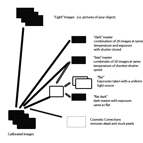
An image is collected as a number of individual exposures (sub exposures) with a particular filter. These are calibrated by removing the effects of reading the CCD (bias), noise due to thermal effects (dark current), and defects in the optical path (e.g. a dust bunnies & vignetting) ("flat"). In early 2012 PI introduced a set of scripts that automates the calibration process. It is now very easy to take your dark and bias masters and use them to calibrate your light images using the flats.While the PI script will also do registration and integration, I do not use this feature. My images require many nights of data before they are complete. I prefer to calibrate nightly or every couple of nights so I can get an idea of the quality of the data (and because I run several observing projects at the same time).
Since my camera now as several dead columns I also am including cosmetic correction in the calibration process.
When I have enough subexposures with enough quality I then build the linear image. The calibrated subexposures are registered (since you move the telescope between frames to improve noise rejection) and then combined. This process includes a number of steps which further reduce the noise in the data.
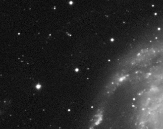
Here are two examples. Click on the images for a larger image. This will allow you to better see what the correction is doing.
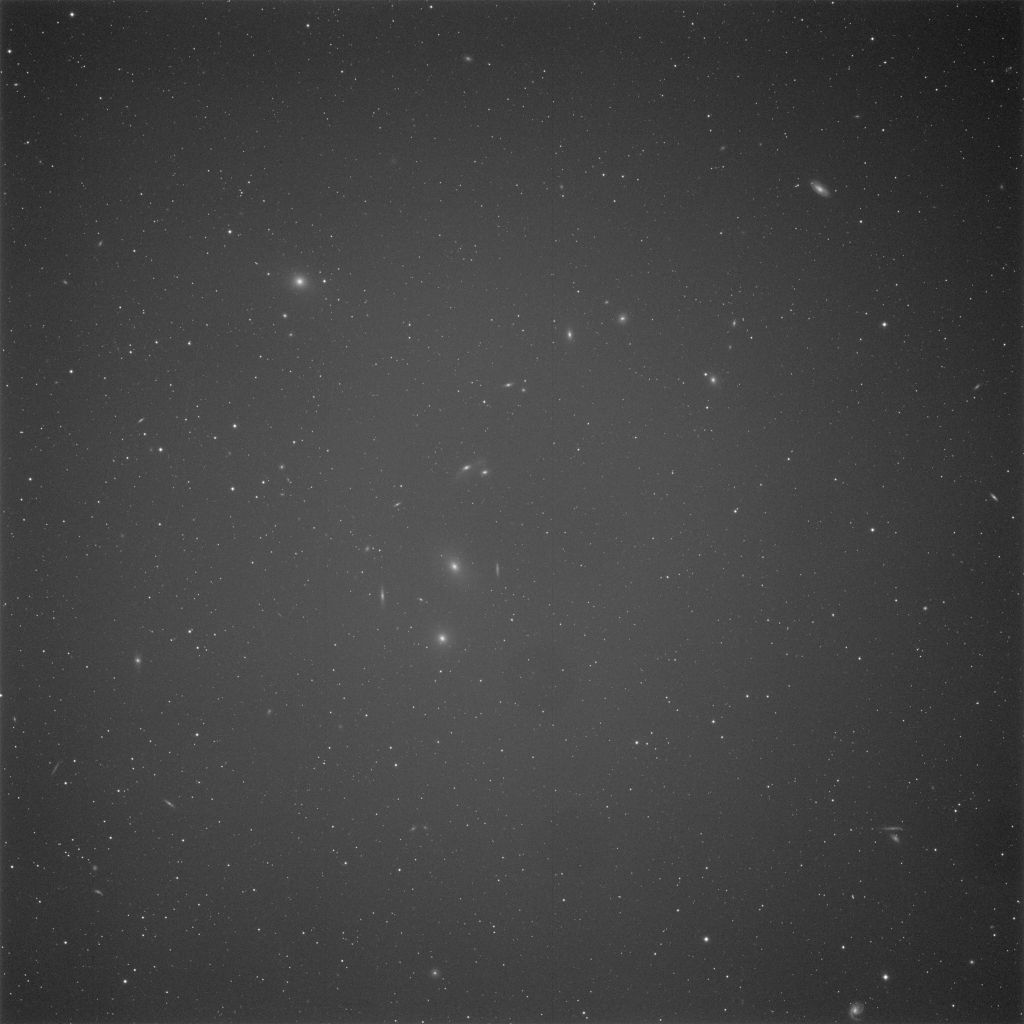
raw |
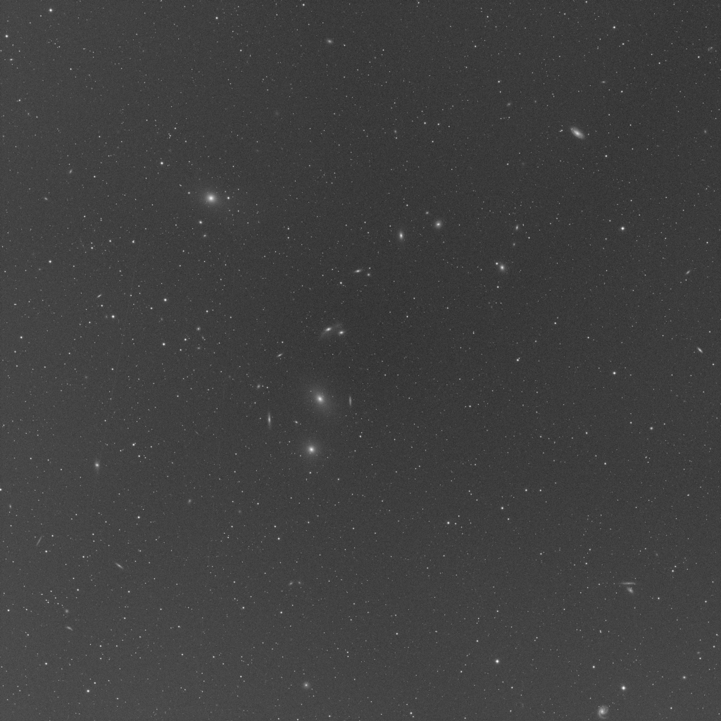
calibrated |
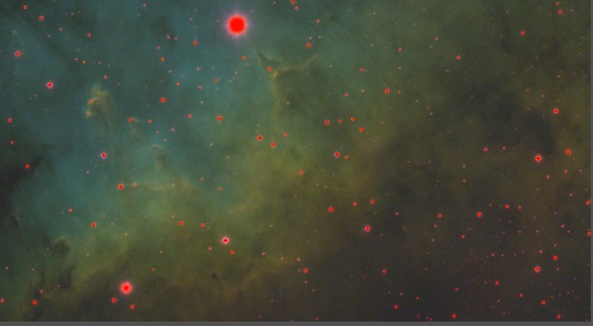
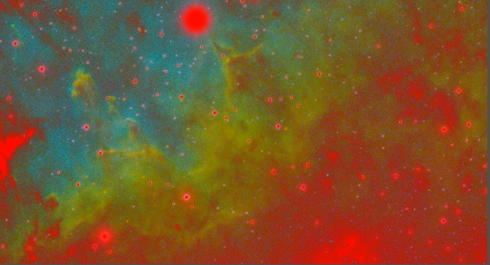
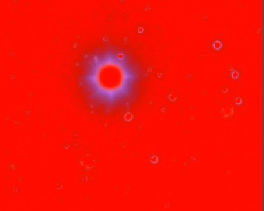
Raw Image
This is what a typical image looks like after calibration. At
this point it is referred to as a linear image. A linear
image is just what the camera captured. Since the intensity
level in the image data is simply divided by to the 256 to obtain
the value for the display intensity, only the brightest stars are
likely visible. No worries your data is there hiding in the
low values (along with the noise). 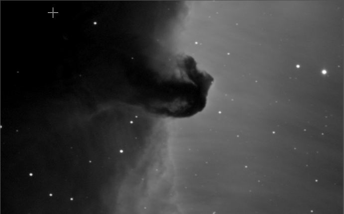
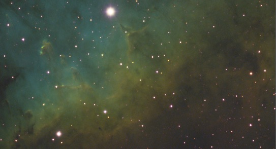
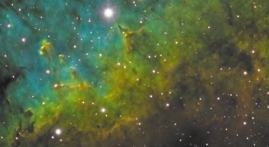
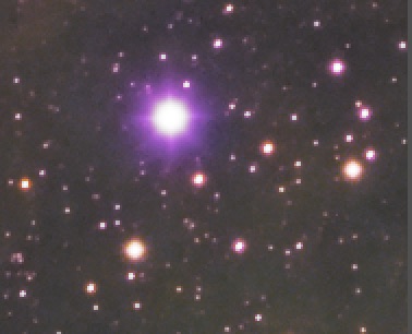
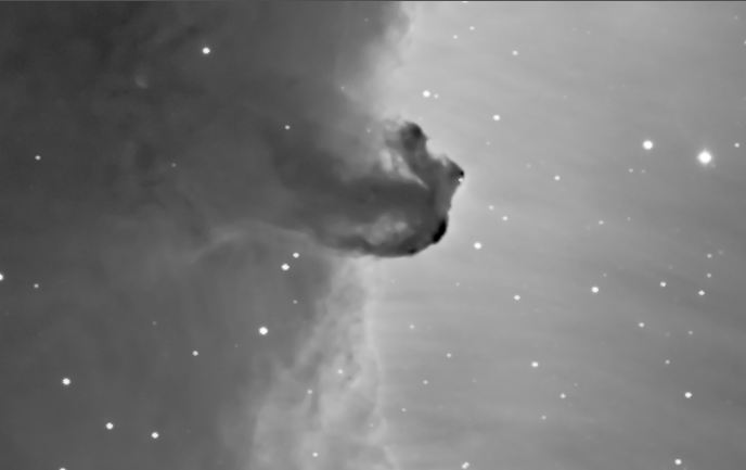
Screen Transfer Function
This is the same image again, but we have used a process called
"Stretching" to reassign the dimmer values to higher display
values. It does this in a way that is nonlinear.
In other words dimmer values are changed more than brighter values.
It is important to note that STF only stretched the displayed image. The underlying data is still linear.

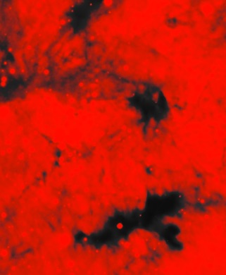
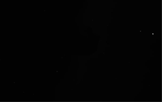
Removing Local
Background
Broadband filters not only record the sky, they also record all of
the junk light. This needs to be removed by a gradient
tool. In PixInsight this is DynamicBackgroundExtraction.
The
image at the left switches from a raw image, to the detected
background, and then to the corrected image. In this image the
gradient was not too bad, but you can see how much was there.
For filters that are very susceptible to light pollution such as a
clear filter I find this needs to be applied to each sub exposure. At Katonah we learned that it is important to place each of the sample points manually. I suggest using a size of something like 10-15 pixels and then manually checking to make sure that each sampled area is really background and that it contains as few stars as possible.
Even my ultra narrowband filters can be subject to gradients. The O III filter is especially susceptible.
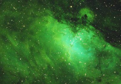
Combining several filters for False (or mostly real) Color
Most of the tutorials for PixInsight are for conventional LRGB images. That is images with a Luminance (or Clear) filter that capture the visual intensity across the entire visible band and R, G, and B filters that capture the color contribution to the Luminance.I don't shoot LRGB due to the local light pollution. Either the NB4Stars or conventional narrowband is built using Channel Combination of the three images. Each filter is assigned a different color channel. It is possible to also assign colors to non-primary colors (e.q. aqua) by applying the value to both green and blue. Using PixelMath one can compose the image any way they want.
Neutralize the Background
Once the images are combined it is likely that the backgrounds of the three images are not set at the same level. Use the Background Neutralization tool to fix this. The image at this point is still going to look pretty ugly. The next two steps will improve that.
Mask Generation
Many Pixinsight processes rely on masks. Masks can be built from either the linear L copy saved above or by extracting the Lfrom the working image. I discuss mask generation in more detail below
Color Calibration
Color Calibration of LRGB images is covered in detail by multiple sources. Even though I never have an L the technique that Vincent taught at Katonah still applies.The ColorCalibration tool then uses this as the white reference. The preview used for the background in the previous step is the background. Turn off structure detection.
This method has several advantages over what I was doing before. Calibrating with a G2V star does not make sense since I typically image over a large part of the sky. Sampling at a single point will not give me the average performance of the camera over the range of elevations I actually used.
The projects we used in examples at Katonah and my own recent M16 project showed that this was both simple and effective. For my narrowband work it prevents Hydrogen from turning the image Green (as can be seen in the beforeimage on the left). It also corrects for my camera being significantly less sensitive to my sV filter than to my other filters.

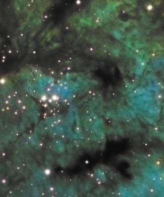
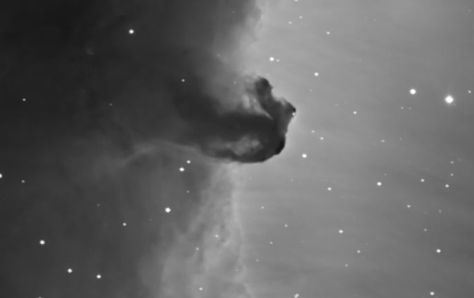
Fix Star Colors
Narrowband images produce stars that have weird halos. This is in part due to to the star sizes appearing to be different with different filters.At the Katonah workshop we were taught to fix this by applying a star mask (see below) and then using Curves to adjust the Saturation so the stars were completely unsaturated. In my work so far I found this worked on some images very well.
The alternative is to extract the L channel from the working image and then overwrite this onto the color image by masking the color image and then using PixelMath to apply the L to the unmasked areas of the color image. This sets the unmasked areas to the intensity of L, but with no saturation (since the RGB values are the same).
In the example note particularly the bright star at the top of the frame.
Linear Noise Removal
Newer versions of the noise tools particularly TGVDenoise are able to be run on linear images. If you are doing this be careful. The defaults are intended for Non-linear images and thus make way too much correction for linear imagesCalculating the true image location
Pixi includes a script "ImageSolver" that will analyze the image and set the FITS header. This is important if you want to add annotation later. In my experience this works better with linear images.Extract the Linear L Channel
Extract the L channel (created internally after RGB Combination). This may be useful in Mask Creation.
Non Linear Stretch
Now it is time to dig into the data and find our image. The Histogram Transformation tool uses a histogram display to reassign the old intensity values to new values.By this point in the process the image is a 32 bit floating point so there is plenty of resolution to work with.
HT will reassign lower intensity values to higher values, but it does so non-linearly. Thus after HT the original low intensity values occupy more of the numeric range than the original high intensity values did.
A trick you can use at this point is to use STF and then drag the triangle of the STF window onto the bottom of an HT window. That will set the HT to the same stretching used in STF. Be sure to hit PF12 to cancel STF on the image before applying the HT.
It is also possible to perform a Masked Stretch. This results in better star images, but cannot be directly used because it does not do enough for the nebulosity. This can be fixed, but describing that process is out of scope for this summary. Consult Harryfor an example.

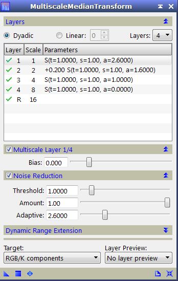
HDR Transform
HDRMT is another tool that is used to remap intensities. HDRMT decomposes the image into layers and finds image structures as a function of their characteristic scales. Basically it forces the intensity levels to spread out and thus give more contrast. Unlike curves it does this based on analysis of the image.HDRMT will tend to dampen the bright areas of the image, but will improve the contrast between the dimmer details and bright stuff. You can recover the brightness in the next step.

Adjust Curves
We learned at Katonah (and later reinforced by Rogelio's walkthrough in IP4AP) it is important at this point to readjust the curves and saturation after HDRMT (and other steps below that flatten the image). This will restore the contrast and make the colors brighter. The CurvesTransform function can separately manipulate the L and the saturation.These steps will require masks which is the subject of the next section.
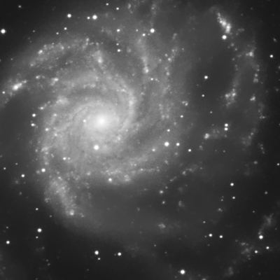
Sharpening
the Image
The MMT
function is the principle tool for sharping (although there
also some similar tools that can also be used). It detects the
wavelets that make up the image and allows you to sharpen and
remove noise at the same time. One sharpens by increasing
the bias of some sizes of structures. The data in this
example was very clean due to the number of exposures used, but
the sharpening and re-emphasis of important structure is dramatic.
It is important that you use a mask when using MMT. At Katonah we learned to protect the stars from sharpening to prevent stars that have unnatural sharp edges.
Noise Reduction
While MMT handles noise in the brighter areas, I have not been satisfied with how it handles the background. The older ACDNR still rocks when it comes to making the background as low in noise as possible, but I have started using TGVDenoise for more recent projects. The latter's controls are sensitive, but when you get them right the results are amazing.
I usually apply different noise reduction to the background than I do to the brighter objects. Create different masks to accomplish this.

Final
Adjustments
Some last minute adjustments are usually needed. Some
combination of these might be needed - more HT - to remap the image to remove pedestal (a constant black level) which sharpens the contrast between light and dark.
- LocalHistogramEqualization - Emphasizes areas of sharply
changing brightness. A more powerful tool than Dark
Structure Enhance.
- Curves - can be used to further improve the contrast and improve color saturation.
- Adding
H
alpha
data Although I typically add this during the linear
portion of the processing.
- Annotating the image with overlays for NGC, etc objects visible